Particular Solution To A Differential Equation
News Co
Apr 05, 2025 · 6 min read
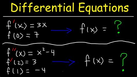
Table of Contents
Finding Particular Solutions to Differential Equations: A Comprehensive Guide
Differential equations are the backbone of many scientific and engineering models, describing the relationships between functions and their derivatives. While finding the general solution provides a family of curves satisfying the equation, often we need a specific solution that satisfies particular initial or boundary conditions. This is where the particular solution comes in. This article delves deep into the methods for finding particular solutions to differential equations, covering various types and techniques.
Understanding Differential Equations and Their Solutions
A differential equation is an equation that relates a function to its derivatives. For example, dy/dx = 2x is a simple differential equation. The general solution represents the entire family of functions that satisfy the equation. For dy/dx = 2x, the general solution is y = x² + C, where 'C' is an arbitrary constant. This constant signifies that infinitely many functions (one for each value of C) satisfy the equation.
A particular solution, however, is a specific member of this family. It's obtained by using initial conditions or boundary conditions to determine the value of the arbitrary constant(s) in the general solution. For example, if we're given the initial condition y(0) = 1, we substitute x = 0 and y = 1 into the general solution y = x² + C to find 1 = 0² + C, which implies C = 1. Therefore, the particular solution is y = x² + 1.
Methods for Finding Particular Solutions
The methods for finding particular solutions depend heavily on the type of differential equation. We'll explore several key approaches:
1. First-Order Differential Equations
First-order differential equations involve only the first derivative of the function. Several techniques exist to solve these, and the choice depends on the form of the equation:
a) Separable Equations:
Separable equations can be written in the form dy/dx = f(x)g(y). The solution process involves separating the variables and integrating both sides:
∫(1/g(y)) dy = ∫f(x) dx
After integration, we obtain the general solution. Applying the initial condition allows us to find the particular solution.
Example: Solve dy/dx = x/y with the initial condition y(0) = 2.
- Separate variables:
y dy = x dx - Integrate: ∫y dy = ∫x dx => (1/2)y² = (1/2)x² + C
- General solution: y² = x² + 2C
- Apply initial condition: 2² = 0² + 2C => C = 2
- Particular solution: y² = x² + 4
b) Linear Equations:
Linear first-order equations have the form dy/dx + P(x)y = Q(x). The solution technique involves finding an integrating factor, I(x) = e^(∫P(x)dx), multiplying the equation by this factor, and then integrating.
Example: Solve dy/dx + 2xy = x with the initial condition y(0) = 1.
- Integrating factor: I(x) = e^(∫2x dx) = e^(x²)
- Multiply equation by I(x): e^(x²) dy/dx + 2xe^(x²)y = xe^(x²)
- Integrate: d/dx [ye^(x²)] = xe^(x²) ∫d/dx [ye^(x²)] dx = ∫xe^(x²) dx
- Solve integral (using substitution u = x²): ye^(x²) = (1/2)e^(x²) + C
- General solution: y = (1/2) + Ce^(-x²)
- Apply initial condition: 1 = (1/2) + C => C = 1/2
- Particular solution: y = (1/2) + (1/2)e^(-x²)
c) Exact Equations:
An exact equation is of the form M(x,y)dx + N(x,y)dy = 0, where ∂M/∂y = ∂N/∂x. The solution involves finding a function F(x,y) such that ∂F/∂x = M and ∂F/∂y = N. The general solution is then F(x,y) = C.
2. Second-Order Linear Homogeneous Differential Equations
These equations have the form ay'' + by' + cy = 0, where a, b, and c are constants. The solution involves finding the characteristic equation and its roots. The particular solution depends on the nature of these roots:
a) Distinct Real Roots:
If the characteristic equation has two distinct real roots, r₁ and r₂, the general solution is y = C₁e^(r₁x) + C₂e^(r₂x). Initial conditions are needed to determine C₁ and C₂.
b) Repeated Real Roots:
If the characteristic equation has a repeated real root, r, the general solution is y = (C₁ + C₂x)e^(rx).
c) Complex Conjugate Roots:
If the characteristic equation has complex conjugate roots, α ± iβ, the general solution is y = e^(αx)(C₁cos(βx) + C₂sin(βx)).
3. Second-Order Linear Non-Homogeneous Differential Equations
These equations are of the form ay'' + by' + cy = f(x), where f(x) is a non-zero function. The solution involves two steps:
-
Finding the complementary solution (y_c): This is the general solution to the associated homogeneous equation (ay'' + by' + cy = 0). The methods described above are used.
-
Finding a particular solution (y_p): This depends on the form of f(x). Techniques include the method of undetermined coefficients and variation of parameters.
a) Method of Undetermined Coefficients:
This method works when f(x) is a polynomial, exponential, sine, cosine, or a combination thereof. We assume a particular solution of a similar form to f(x) and then determine the coefficients by substituting into the original equation.
b) Variation of Parameters:
This method is more general and works for any f(x). It involves expressing the particular solution as y_p = u₁(x)y₁(x) + u₂(x)y₂(x), where y₁ and y₂ are linearly independent solutions to the homogeneous equation, and u₁ and u₂ are functions determined using a specific formula involving integrals.
4. Higher-Order Differential Equations
The principles extend to higher-order equations. The general solution will involve more arbitrary constants, which are determined using more initial or boundary conditions. The methods for finding particular solutions often become more complex, relying heavily on linear algebra techniques.
Importance of Particular Solutions in Applications
Particular solutions are crucial in various applications:
-
Physics: Determining the trajectory of a projectile, analyzing the motion of a damped harmonic oscillator, understanding the behavior of electrical circuits.
-
Engineering: Designing structures that can withstand specific loads, modeling the flow of fluids in pipes, optimizing control systems.
-
Biology: Modeling population growth, simulating the spread of diseases, analyzing chemical reactions in biological systems.
-
Economics: Predicting economic trends, forecasting stock prices, analyzing the impact of government policies.
Conclusion
Finding particular solutions to differential equations is a fundamental skill in many scientific and engineering disciplines. The choice of method depends on the type and form of the equation, and mastering these techniques is essential for accurately modeling and understanding real-world phenomena. This comprehensive guide has provided a solid foundation for understanding and implementing various methods to successfully obtain particular solutions, transforming theoretical models into concrete, meaningful predictions and analyses. Remember that practice is key—working through various examples and exercises will solidify your understanding and build your problem-solving skills.
Latest Posts
Related Post
Thank you for visiting our website which covers about Particular Solution To A Differential Equation . We hope the information provided has been useful to you. Feel free to contact us if you have any questions or need further assistance. See you next time and don't miss to bookmark.